
Demographic Risk Factors of COVID-19
Introduction
The disproportionate effects of COVID-19 across the United States have highlighted long-standing health and social disparities that put certain demographic groups at high risk of contracting and/or experiencing the worst outcomes of the virus. Here, we examine a spectrum of key demographic variables and their importance in determining COVID-19 disease dynamics on a county level during the period of April 1, 2020 to May 1, 2020.
Methods
Data Sources
Raw Data Sources Population density data was calculated from total population data from Annual County Resident Population Estimates by Age, Sex, Race, and Hispanic Origin: April 1, 2010 to July 1, 2018 from the U.S. Census Bureau [1] and land area data from TIGERweb State-Based Data Files [2].
Demographic data on age, sex, and race were obtained from Annual County Resident Population Estimates by Age, Sex, Race, and Hispanic Origin: April 1, 2010 to July 1, 2018 from the U.S. Census Bureau, Population Division [1]. Only 7/1/2018 population estimates were used. Data on median income, health insurance, poverty status, and educational attainment were obtained from the 2018 ACS 5-year Estimates from the U.S. Census Bureau [3]. Unemployment data were obtained from 2018 Local Area Unemployment Statistics (LAUS) from the U.S. Bureau of Labor Statistics [4].
Data on cardiovascular disease, diabetes, and obesity were obtained from the National Center for Chronic Disease Prevention and Health Promotion, Division for Heart Disease and Stroke Prevention’s Interactive Atlas of Heart Disease and Stroke [5]. COVID-19 case and death data from 4/1/2020 to 5/1/2020 were obtained from USAFacts’ COVID-19 issue page [6]. The health conditions included in this study were selected due to their prevalence as co-morbidities for COVID-19 patients.
Data Analysis
Some variables within the same demographic category were removed to correct for multicollinearity in the data — multicollinearity is defined as incidents when there are high correlations between two or more predictor variables, which can skew the results in a regression model. In our analysis, since sex, race, and age were represented as percentages, at least one variable in each was left out to prevent multicollinearity which manifested as NA values in the fitlm() output, e.g. percent female was removed and only percent male was used to represent sex.
Since the aim of the study was to determine demographic variables’ influence on COVID-19 dynamics, we removed all counties with 0 values for case or death counts from the data set before analysis.
Analysis was performed using fitlm() for regression, pca() for principal components analysis and regression, and fsrftest() for feature selection in MATLAB R2019b.
Results
Multiple Regression Analysis
Multiple regression is a common technique used to model how multiple independent predictor variables impact a dependent variable. The coefficient of each predictor in the model is interpreted in the context of all other variables held constant, and thus the importance of the predictors relative to the dependent variable can be compared. We used multiple regression analysis here to discern which of the predictor variables have strong associations with COVID-19 disease dynamics.
Using an alpha level of 0.05, we found that population density, sex, race, age distributions, socioeconomic factors, and diabetes and obesity prevalence were all significantly correlated with COVID-19 incidence.
Using an alpha level of 0.05, we found that population density, sex, race, age distributions, socioeconomic factors, and diabetes and obesity prevalence were all significantly correlated with COVID-19 incidence. Among these factors, population density had the lowest coefficient p-value and the smallest coefficient, indicating that population density had little predictive power for disease incidence in the county data. In terms of statistical significance, population density was followed by percent completed high school, percent without health insurance, and percent American Indian and Alaska Native alone. All of the statistically significant predictors had coefficients of less than 0.02, indicating little predictive power.
Using the same threshold for significance, we found that population density, sex, race, age, socioeconomic factors (excluding percent completed high school), and cardiovascular disease death rate were significantly correlated with COVID-19 death rate.
Using the same threshold for significance, we found that population density, sex, race, age, socioeconomic factors (excluding percent completed high school), and cardiovascular disease death rate were significantly correlated with COVID-19 death rate. Population density had the lowest p-value by several orders of magnitude followed by median household income and percent over 65 years old, but all statistically significant predictors had coefficients less than 10-4, indicating very little predictive power.
The incidence and death rate regression models had R-squared values of 0.174 and 0.24 respectively. These low R-squared values were somewhat expected since we hypothesized that variables like disease infectiousness, contact frequency, and quality of healthcare might more directly determine disease dynamics as they are traditionally incorporated in compartmental disease models. We also knew that there would be high variation between counties since the time frame of the data was relatively early on in the pandemic and many rural counties had very low case counts. These prior assumptions about the model also helped us reason why the correlation coefficients were so low.
Since the data used for this analysis was from relatively early in the course of the pandemic in the US, it was heavily skewed. Many counties had not yet had an index case (these were removed from the dataset), and among those that did, disease dynamics varied widely between those with significant outbreaks and those with isolated cases and little spread. For this reason, we chose to log-transform the incidence and death rate data for further regression analysis.
In the log-transformed results, population density, race, socioeconomic factors, diabetes and hypertension were significantly correlated with log of incidence. Of these factors, race had the greatest predictive power with coefficients up to 0.25. Interestingly, sex and age did not correlate with incidence after log transformation.
Population density, sex, percent over 65 years old, race, socioeconomic factors, and cardiovascular disease death rate were significantly correlated with log-transformed death rate. Race again had the greatest predictive power of these variables with coefficients up to 0.14.
The R-squared values of the log-transformed incidence and death rate regression models were 0.24 and 0.19 respectively. Again, the low R-squared values were somewhat expected for the aforementioned reasons.
Principal Component Regression
Since our dataset encompassed many variables, we also performed principal component regression (PCR) to explore whether through dimension reduction a combination of these explanatory variables could more efficiently and powerfully predict COVID-19 incidence and death rate. PCR is a regression technique that correlates the dependent variable with the principal components of the explanatory variables rather than the explanatory variables themselves, and is especially useful for overcoming multicollinearity amongst the explanatory variables and reducing dimensionality by characterizing the model in fewer parameters.
From an elbow plot of percent variance explained by each principal component (PC), we selected PCs 1 through 4 for regression analysis. We also included the lowest variance PCs, 17 and 18, since the PCs capturing low variance can be important in PCR.

The PC loadings of our selected components reveal the weights of the explanatory variables in contributing to each PC, i.e. which variables are important to this component. We found that PC1 was loaded heavily in socioeconomic factors, health conditions, and race; PC2 was loaded heavily in race, age, and population density; PC3 was loaded heavily in race, age, population density, and sex; PC4 had large loadings for almost every variable. PC17 had high loadings for income and poverty prevalence, and PC18 was loaded almost entirely by race.

We continued to use the log-transformed incidence and death rate data for PCR with the same reasoning as in multiple regression.
All of the linear regressions between PCs and disease dynamics had significant p-values but very small correlation coefficients due to high scatter in the data. The low R-squared values indicate low explaining power; in context, we expected this result since predictors that are known to determine disease dynamics like contact rates, availability of treatment, and public health interventions were not included in the model.
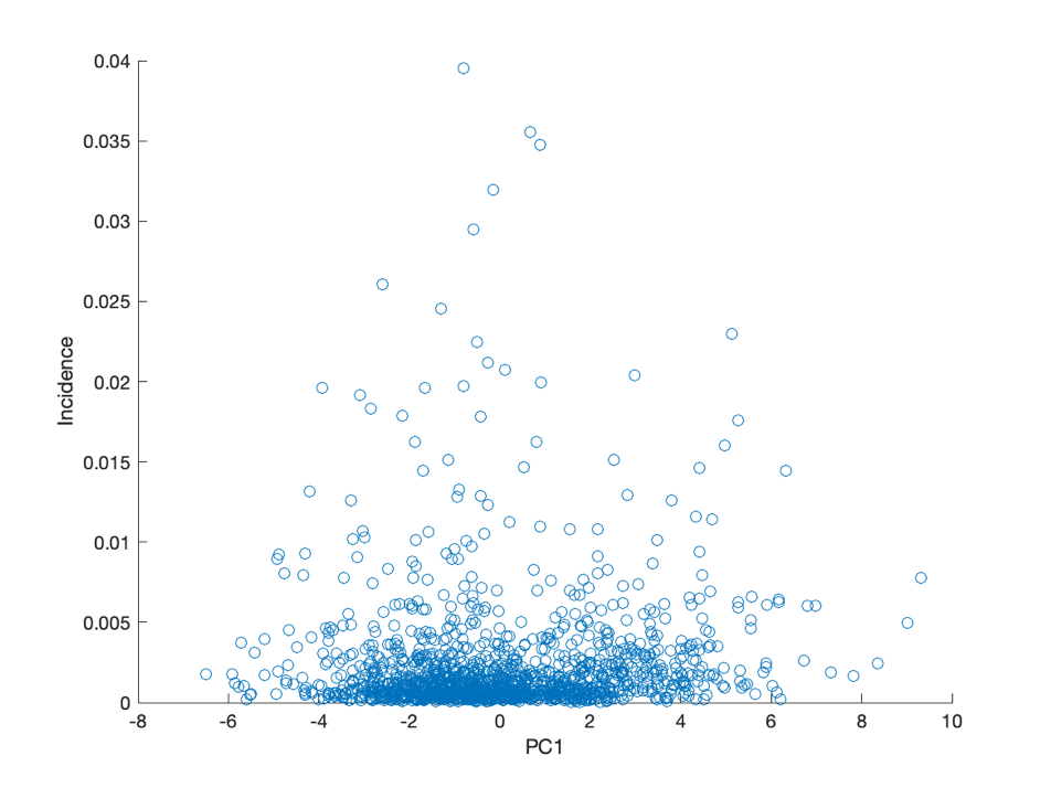

Top Row: Incidence PC1, PC2, PC3, PC4
Bottom Row: Death Rate PC1, PC2, PC3, PC4

Top Row: Incidence PC17, PC18
Bottom Row: Death Rate PC17, PC18
Feature Selection
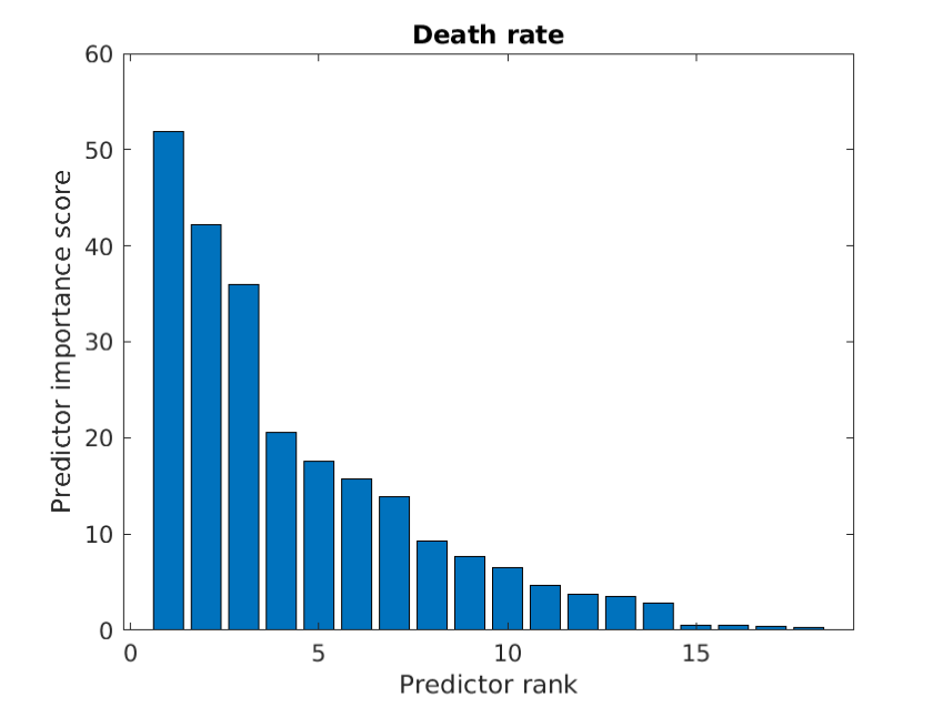
One final perspective on these demographic variables’ importance to COVID-19 we investigated was in feature selection, which reveals which predictor variables are most important for modeling a chosen response variable.
For incidence, the top 5 predictors were population density, percent white, percent black, percent completed high school, and percent male.
For incidence, the top 5 predictors were population density, percent white, percent black, percent completed high school, and percent male. For death dynamics, the top 5 predictors, with a notable drop in importance between the third and fourth predictors, were population density, percent white, percent black, median household income, and percent male.
For death dynamics, the top 5 predictors, with a notable drop in importance between the third and fourth predictors, were population density, percent white, percent black, median household income, and percent male.
These feature selection results corroborate the importance of population density, race, and level of education in determining incidence and the importance of population density, race, and income in determining death rate as revealed in the multiple regression outputs and PCR.

Discussion
Our analysis provides quantitative confirmation on a county level of reported broader demographic-based trends in the pandemic. We utilized PCA to reduce the dimensionality and solve potential collinearity among chosen independent variables to investigate important combinations of demographic variables that might make certain populations particularly vulnerable. COVID-19 has disproportionately hurt indigenous, colored, and under-resourced communities, and here we show how the geographic, racial, and socioeconomic characteristics of these communities are interconnected in determining the disease’s impact. These factors are linked, and in combination shape how different groups are experiencing and reacting to the pandemic. It is crucial to consider the role that these demographic factors play in population vulnerabilities in making policy initiatives to address COVID-19 and future health crises.
References
U.S. Census Bureau, Population Division. (2019). Annual County Resident Population Estimates by Age, Sex, Race, and Hispanic Origin: April 1, 2010 to July 1, 2018 [Data file]. Retrieved from https://factfinder.census.gov/bkmk/table/1.0/en/PEP/2018/PEPASR6H?#
U.S. Census Bureau. (2019). Counties - ACS 2018 (Data as of January 1, 2019) [Data files]. Retrieved from https://tigerweb.geo.census.gov/tigerwebmain/TIGERweb_counties_acs18.html
U.S. Census Bureau. (2019). 2018 ACS 5-year Estimates [Data files]. Retrieved from https://www2.census.gov/programs-surveys/acs/summary_file/2018/data/5_year_geographic_comparison_tables/?C=D;O=A
U.S. Bureau of Labor Statistics. (2019). Labor force data by county, 2018 annual averages [Data file]. Retrieved from https://www.bls.gov/lau/laucnty18.xlsx
National Center for Chronic Disease Prevention and Health Promotion, Division for Heart Disease and Stroke Prevention. (2020). Interactive Atlas of Heart Disease and Stroke [Data files]. Retrieved from https://nccd.cdc.gov/DHDSPAtlas/?state=County
USAFacts. (2020). Coronavirus Known Cases, Deaths [Data files]. Retrieved from https://usafacts.org/visualizations/coronavirus-covid-19-spread-map/
This article reports the work of Harvard College Data Analytics Group’s Summer Think Tank. Our Healthcare team, who authored this article, focused on researching healthcare-related aspects of COVID-19.
Edited by Kelsey Wu.